


Partitioning Data in Distributed Systems
Chapter 6 of Designing Data Intensive Applications: Partitioning

Welcome to the 10% Smarter newsletter. I’m Brian, a software engineer writing about tech and growing skills as an engineer.
If you’re reading this but haven’t subscribed, consider joining!
Last week, we explored the replication of data in distributed systems. Today we’ll look into partitioning, a similar practice which is the splitting up of data to increase scalability. Let’s get started!
Partitioning
Partitioning, also known as sharding, is the practice of breaking up data into smaller chunks of the data called partitions. Each record belongs to exactly one partition, but may still be stored on several nodes for fault tolerance. A node may store more than one partition.
Partition data increases scalability. Query load can be distributed across many processors. Throughput can be scaled by adding more nodes.
The goal of partitioning is to spread the data and query load evenly across nodes. If a partition is unfair, we call it skewed. A partition with disproportionately high load is called a hot spot. You can't avoid hot spots entirely.
It's the responsibility of the application to reduce the skew. A simple technique is to add a random number to the beginning or end of the key.
How Should You Partition Data?
There are two ways to partition by data: you can partition by key range or partition by hash of key.
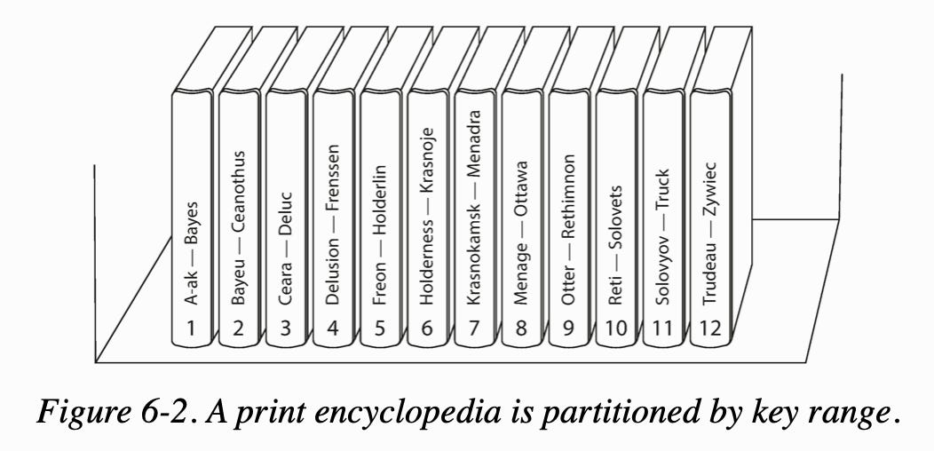
In partition by key range, you assign a continuous range of keys. Like an encyclopedia, you can search based on index key and range scans, such as find all records that start with 'a,' are easy.
The downsides are that some access patterns can lead to hotspots. An example is if the key is timestamp, all writes for today will go to the partition handling today's timestamp. Instead, you can choose to partition by something else like client id.
In partition by hash key, a good hash function takes skewed data and makes it uniformly distributed. It does not have to be cryptographically strong (MongoDB uses MD5). Each partition is assigned a range of hashes which can be evenly spaced by pseudorandomly with consistent hashing.
The downside is we can no longer do efficient range queries.
Partitioning With Secondary Indexes
Partitioning with Secondary Indexes similarly has two strategies. You can either partitioning secondary indexes by document or partitioning secondary indexes by term.
In partitioning secondary indexes by document, each partition maintains its secondary indexes, covering only the documents in that partition (local index). This requires sending a query to all partitions and combining the results (scatter/gather). This is prone to tail latency amplification but is widely used in MongoDB, Cassandra, and Elasticsearch.

In partitioning secondary indexes by term, we construct a global index that covers data in all partitions. The global index must also be partitioned so it doesn't become the bottleneck. This is also called term-partitioned because the term we're looking for determines the partition of the index. Reads become more efficient as rather than a scatter/gather over all partitions, a client only needs to make a request to the partition containing the term that it wants. The downside of a global index is that writes are slower and complicated.

Rebalancing Partitions
Rebalancing partitions is the process of moving load from one node in the cluster to another.
Some strategies for rebalancing are:
How not to do it: Hash mod n. The problem is if the number of nodes N changes, most of the keys will need to be moved from one node to another.
Fixed number of partitions. Create many more partitions than there are nodes and assign several partitions to each node. If a node is added to the cluster, we can steal a few partitions from every existing node until partitions are fairly distributed once again. The number of partitions does not change, nor does the assignment of keys to partitions. The only thing that change is the assignment of partitions to nodes.
Dynamic partitioning. The number of partitions adapts to the total data volume. An empty database starts with an empty partition. While the dataset is small, all writes have to processed by a single node while the others nodes sit idle.
Partitioning proportionally to nodes. Have a fixed number of partitions per node. This approach also keeps the size of each partition fairly stable. This is used by Cassandra.
Sometimes it’s good to do manual partition rebalancing. Fully automated rebalancing may overload the network or the nodes and harm the performance of other requests while the rebalancing is in progress. It can be good to have a human admin in the loop doing rebalancing. This helps avoid operational surprises.
What is Request Routing?
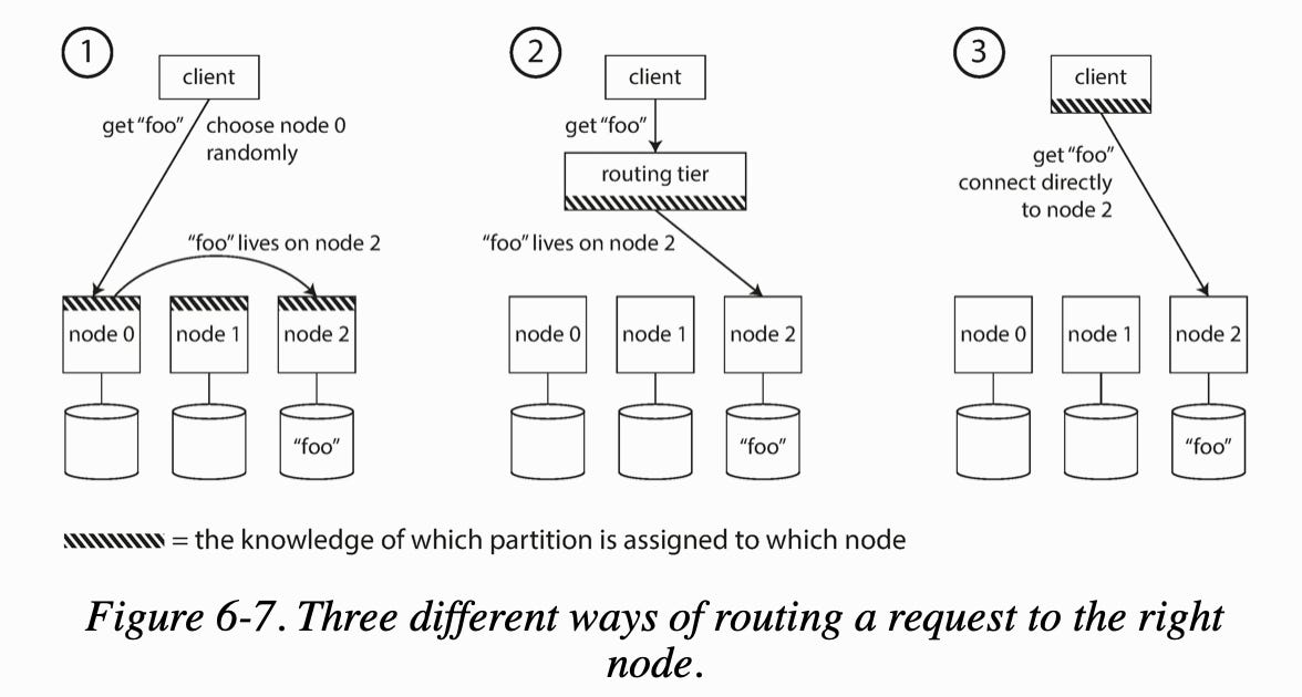
Request routing solves the problem of when a client wants to make a request, it does not know which node to connect to.
Approaches to solve this problem include:
Allow clients to contact any node and make them handle the request directly, or forward the request to the appropriate node.
Send all requests from clients to a routing tier first that acts as a partition-aware load balancer.
Make clients aware of the partitioning and the assignment of partitions to nodes.
Many distributed data systems rely on a separate coordination service such as ZooKeeper to keep track of this cluster metadata. Each node registers itself in ZooKeeper, and ZooKeeper maintains the authoritative mapping of partitions to nodes. Cassandra uses a different approach: they use a gossip protocol that spread routing metadata quickly among the cluster.

Conclusion
This covers the practice of partitioning data in a distributed system, and the two ways of doing so through key range and key hash. Stay tuned as transactions and different isolation levels are next. Feel free to share this article if you liked it!